In our "Used Cars Price Prediction" project, our objective was to create a machine-learning model utilizing linear regression. We began by conducting exploratory data analysis and feature engineering to the dataset we gathered through web scraping. Our data was available from arabam.com, a regional platform selling used cars. Web Scraping
Tools
For our workspace, we utilized Jupyter Notebook. To scrape data from arabam.com, we employed Requests and BeautifulSoup. Numpy and Pandas can transform the gathered data into a structured data frame.
Preliminaries
Our initial step involved creating a "getAndParseURL" function, which will be instrumental in sending requests to websites in the subsequent stages of our project.

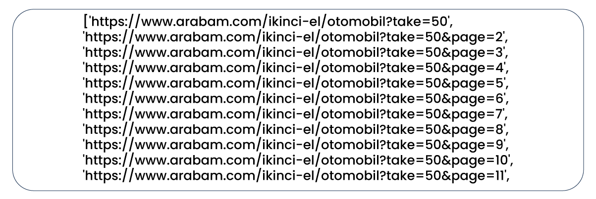
Next, we assembled the links to the web pages that list the data we intend to scrape.

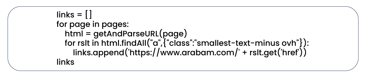
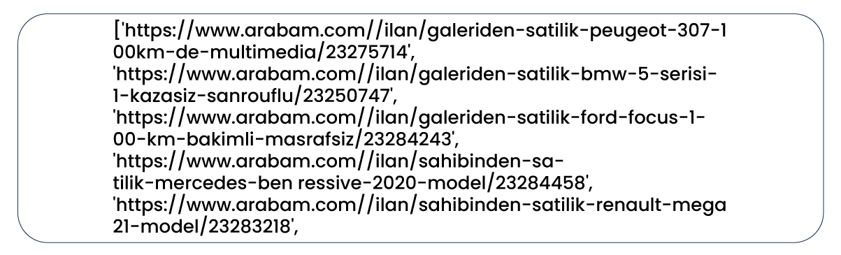
We have compiled a list of all the advertisement links on each previously collected page. It allows us to use a for loop to send requests to each link.
Scraping
Now, it's time to perform web scraping car data. Within our for loop, we instructed the program to retrieve each car feature from every car advertisement and add it to our result list as a variable. We then converted this list into a data frame. Additionally, if the program encounters difficulty accessing the data of a particular feature, it will assign the value of that variable as NaN.
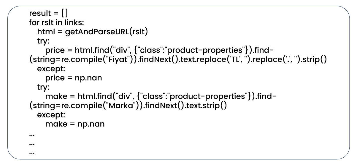
Given that our links list contains 2,500 links and we aim to scrape 22 features from each link, we should anticipate a resulting data frame with 2,500 rows and 22 columns.
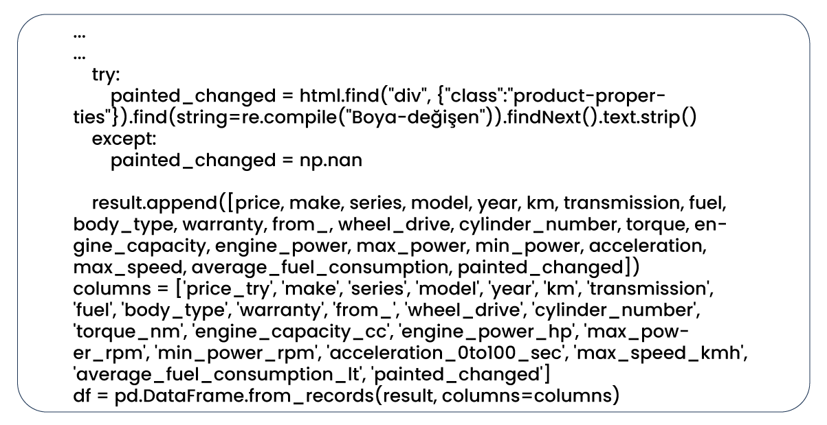
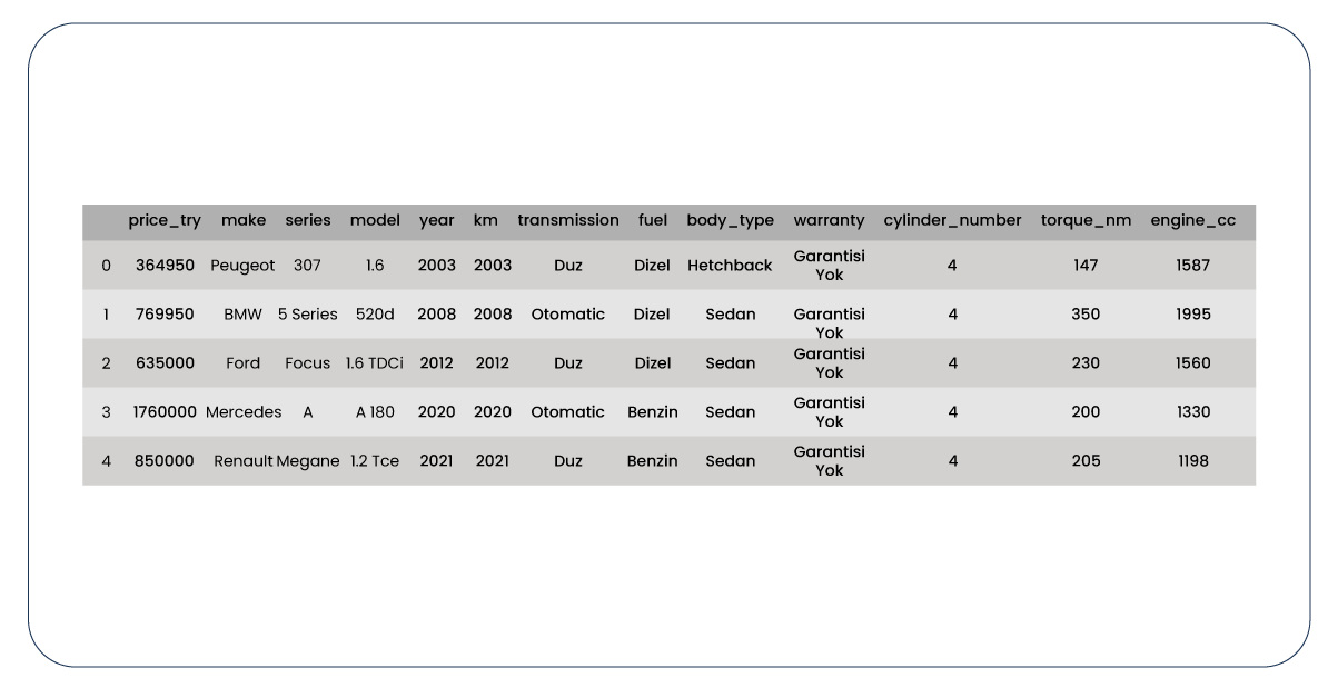
Here is a representation of what our data frame looks like.
In the final step, we moved the last 1000 rows from our data frame into a new one, specifically for the prediction phase of our machine learning model. Subsequently, we saved both of these data frames as CSV files.

Cleaning and Transforming Numeric Data
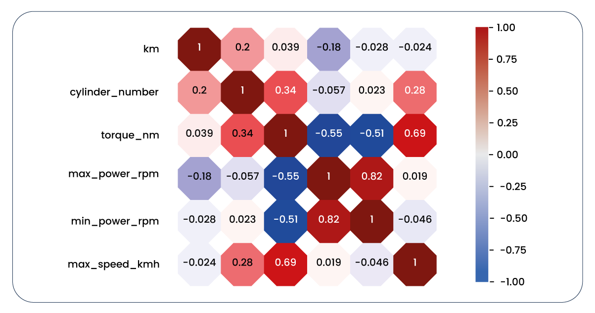
Upon importing our datasets and saving them as CSV files, our initial step involved inspecting all our columns and assessing the correlation values among our numeric columns. However, we encountered an issue where specific columns, expected to contain numeric values, were identified as having an object data type. It was not the expected data type.
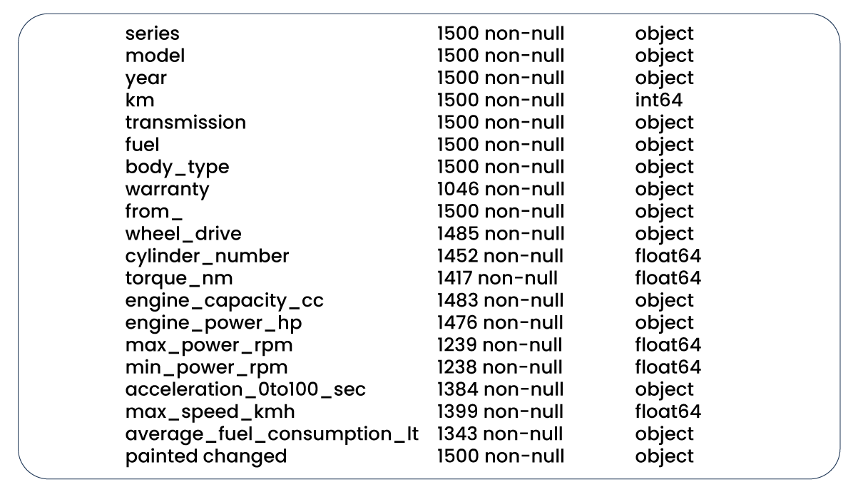
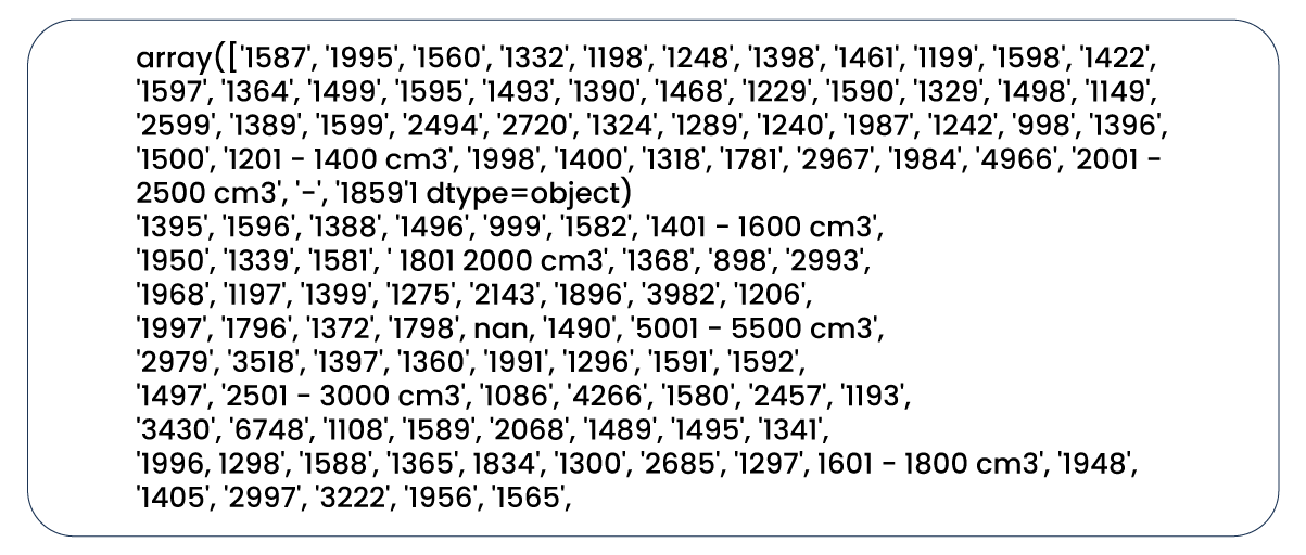
Let's examine the unique values in the "engine_capacity_cc" column.
We need to perform a series of edits to convert the values within this column to the integer data type. First, we'll extract only the numeric components from all values using Pandas's "extract()" function.

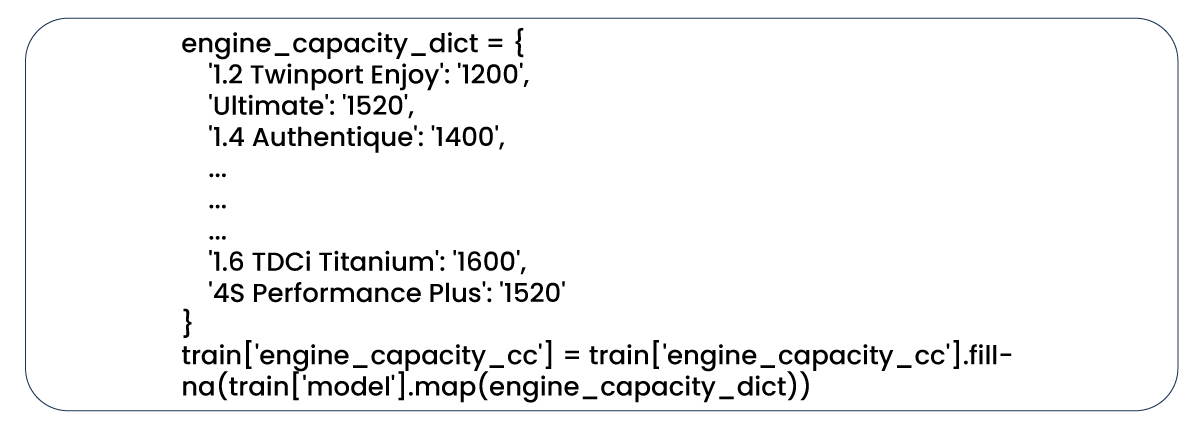
When attempting to change the column's data type to an integer using the "astype()" method in Pandas, we encountered an error due to the presence of null values in our column. These null values are inconvertible to an integer data type. After thoroughly examining the other columns, we have determined that utilizing the "model" column is most appropriate to fill in the null values within the "engine_capacity_cc" column. We manually created a dictionary to achieve this and employed Pandas' "map()" function.
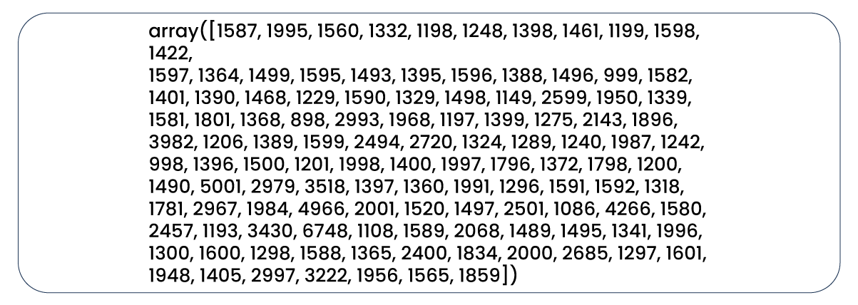
Now, it's evident that all values in our column are in the integer data type.
Let's examine the unique values in the "cylinder_number" column.

After researching the Internet, we discovered that the number of cylinders correlates with engine capacity. With this insight, we implemented a for loop to populate the null values in our "cylinder_number" column accordingly.
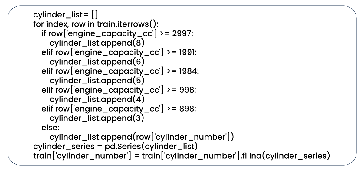
Subsequently, we utilized the "astype()" function to convert all the values in our column to the integer data type.
-function-to-convert-all-the-values-in-our-column-to-the.png)
For the "year" and "price_try" columns, minimal editing was required, primarily involving converting their values to the integer data type.


Considering that the other columns containing numeric values are available due to their correlations, I won't delve into their specifics here to keep the article concise and engaging. You can explore the full notebook on my GitHub repository, which I will provide at the end of this article.
Now, let's focus on the categorical data within our columns, as there are quite a few.
We'll begin with the "make" column. The brand of a car is a crucial factor in determining its price. However, given the multitude of brands in our dataset, we decided to group some of them under the label 'other' to prevent an excessive proliferation of columns when we create dummy variables.

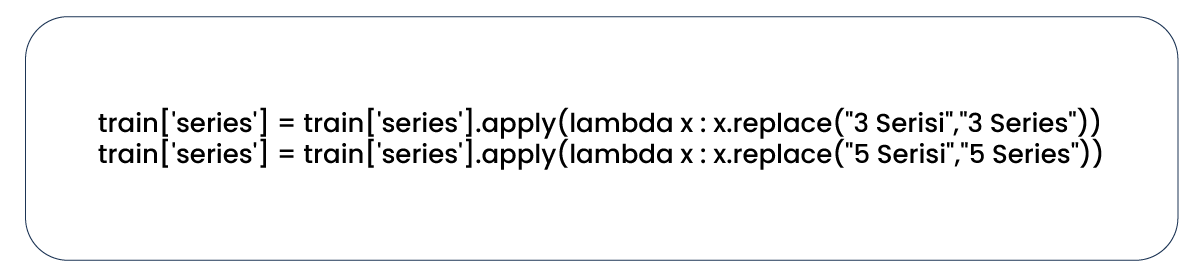
In the "series" column, we've amalgamated specific values under the 'other' category. However, we implemented an additional adjustment to indicate which series belongs to which brand. Additionally,
we translated specific Turkish values into English for clarity.


The "model" column, which we utilized to fill the null values in the "engine_capacity_cc" column, also contains an excessive number of unique categorical values. It, in turn, leads to the 'too many columns' issue when generating dummy variables. Moreover, given that much of the information in other columns is closely related to the values in this column, we have decided that retaining the "model" column is no longer necessary.

We encountered analogous issues with the other columns comprising of categorical values and addressed them using a similar approach. In some cases, we translated Turkish values into English; in others, we grouped specific values under the 'other.' We filled null values with the most frequent value in a few instances, as we couldn't establish a meaningful relationship with other columns or variables. To avoid redundancy, I won't elaborate on each case here, but you're welcome to explore the complete details in my notebook.
Ultimately, we removed duplicate rows from our dataset and saved it as a CSV file for utilization in the feature engineering phase. We executed similar procedures for the test dataset, except for excluding the "price_try" column, which won't be helpful in the prediction phase.
Let's take a closer look at our expected outcomes.
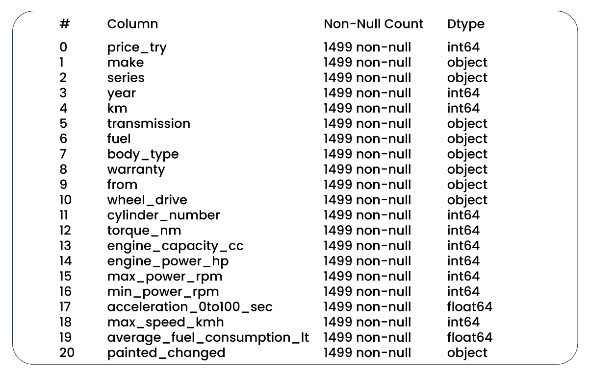
Now, let's delve into feature engineering, where we elevate our analytical and coding prowess to a higher level. We imported our datasets from "arabam_train.csv" and "arabam_test.csv" files and initiated training with a simple linear regression model. Our target variable was the "price_try" column, and the features considered were "year," "km," and "engine_capacity_cc." However, as anticipated, our initial model yielded a meager R-squared score, indicating that significant work lay ahead.
Our initial investigation focused on the distribution of the "year" column. While it could be better, it appears manageable, too.
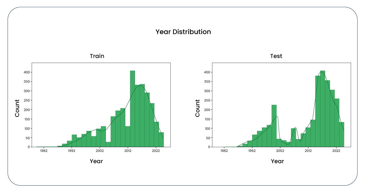
To facilitate scaling, we transformed the "year" column into "age." As a result, we observed a similar graph, albeit inverted.

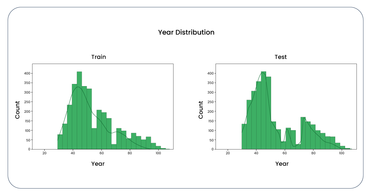
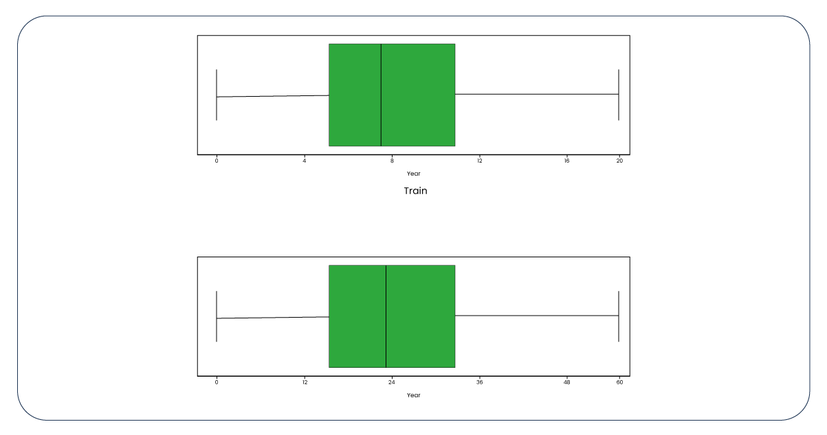
Now, let's examine boxplots to identify potential outliers.
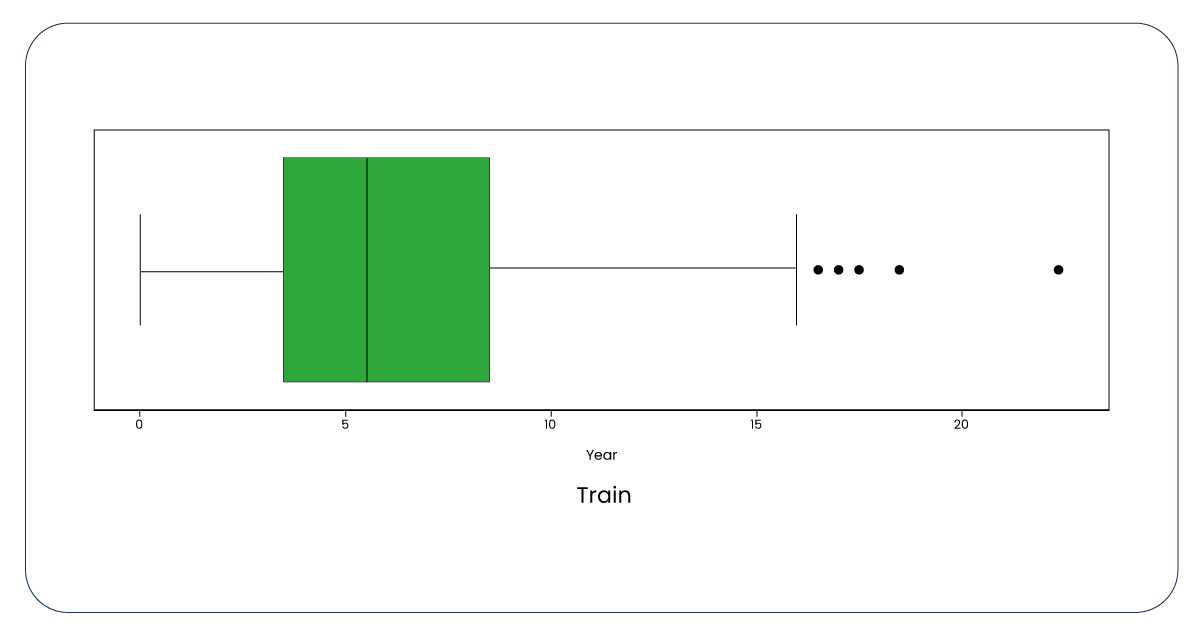
The presence of outliers is not negligible in our data. To determine the boundaries for these outliers, we have established a function with the upper quartile set at 75 and the lower quartile at 25.
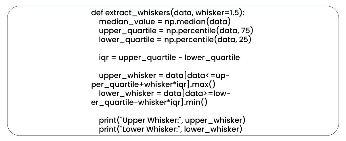
Upon applying the function to the "year" column, we determined that the upper whisker is 32 and the lower is 0. Subsequently, by removing rows where the "year" column is less than 32 from the training dataset, we observed a reduction in the number of rows from 1,499 to 1,479. A similar adjustment was made to the test dataset, reducing it from 999 to 989 rows. This reduction in dataset size is considered acceptable, and now, let's revisit the boxplots and distributions, which exhibit notable improvement.
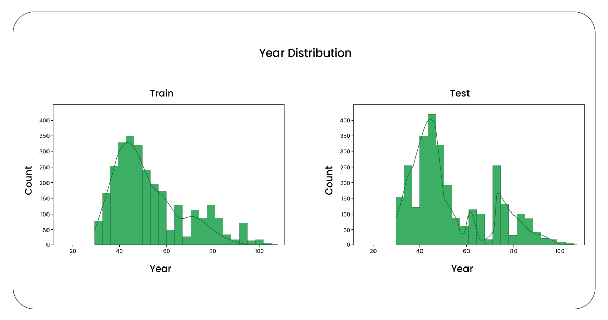
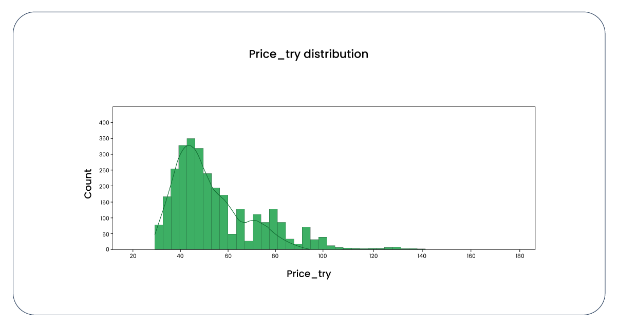
Now, let's examine the distribution of values in the "price_try" column, which is exclusive to our training dataset. Here, we observe a positive skew in the data.
We applied the logarithm function to all the values to mitigate the skewness. This adjustment has resulted in a negative skew, an improvement compared to the previous positively skewed distribution.

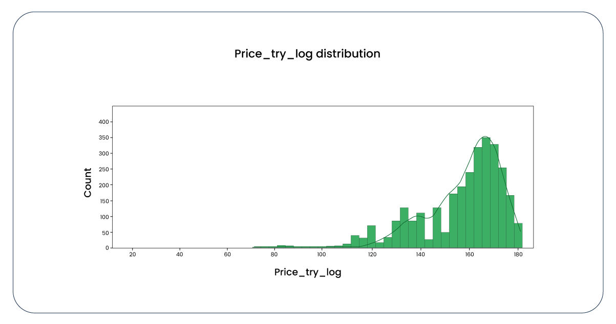
We performed analogous operations on other columns containing numeric values, including whisker removal and logarithmic transformations. We sometimes applied both operations as needed, leaving some columns unaltered. It's important to note that extracting whiskers in specific columns would lead to losing unique values. Please refer to my complete notebook for a comprehensive view of these operations.
Now, let's revisit the correlation heatmap of our columns containing numerical values.
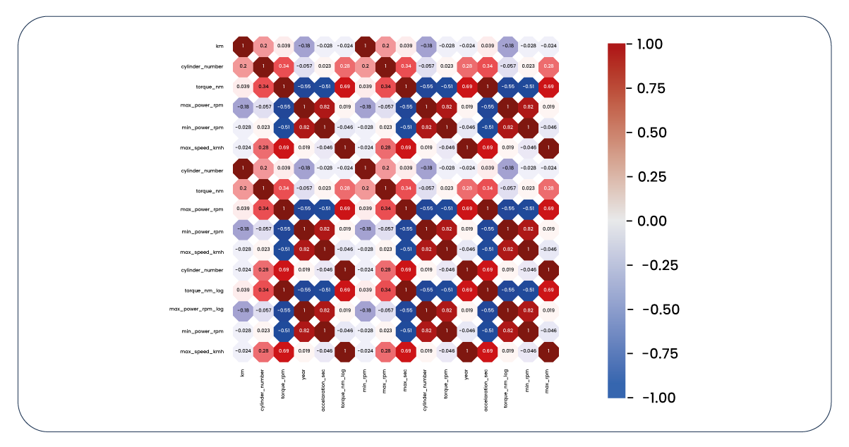
The updated correlation heatmap is considerably more significant than the initial one. However, it reveals several issues. Some features exhibit minimal impact on our target variable, while others have such negligible influence that they aren't practically useful. Furthermore, there are positive and negative correlations between certain features, raising concerns about multicollinearity. To address these issues, we must bid farewell to the columns exhibiting these problems.
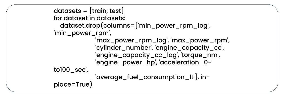
The situation has improved with the removal of problematic columns.
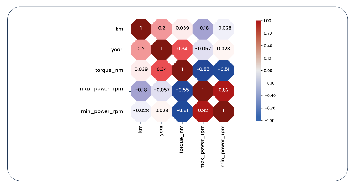
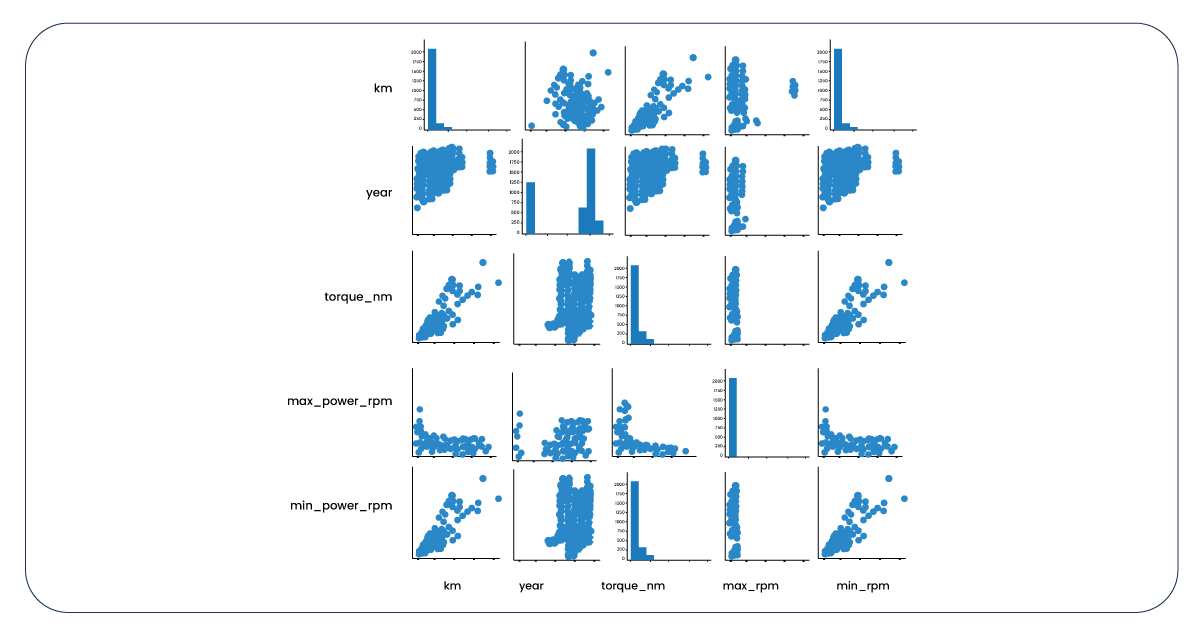
Now, let's examine the same information from an alternative viewpoint.
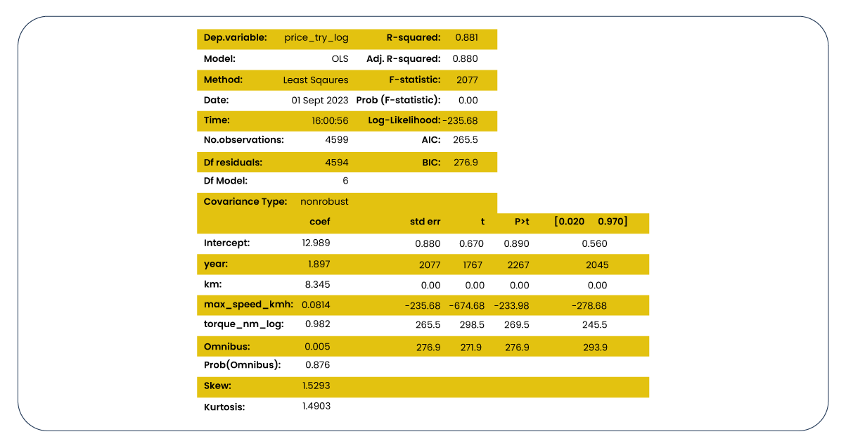
Next, let's analyze the OLS Regression Results generated through statmodels. At this stage, our primary focus is ensuring the R-squared and Adj. R-squared scores are both high and closely aligned. Furthermore, low p-values are crucial, indicating that the relevant features are not affecting the target by chance.
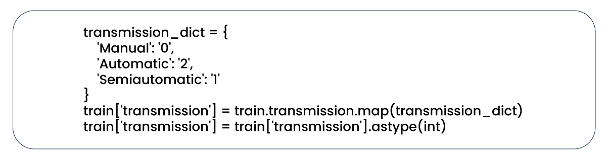
Now, it's time to transform categorical data useless in machine learning modeling into numerical data. We will employ label encoding for columns having categorical data that exhibit a hierarchical or dominant relationship. Let's take the "transmission" column as an illustrative example.
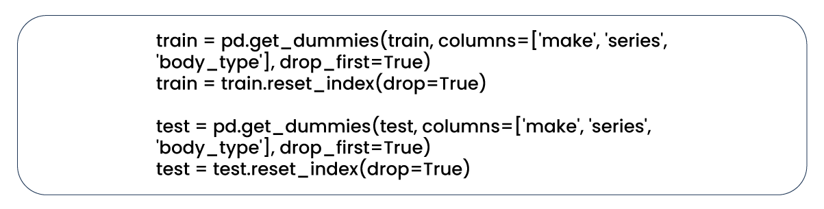
We employed label encoding for most of our categorical features in both datasets. However, for "make," "series," and "body_type" features, it was more appropriate to create dummy variables using one-hot encoding.
Let's revisit our correlation heatmap once more.
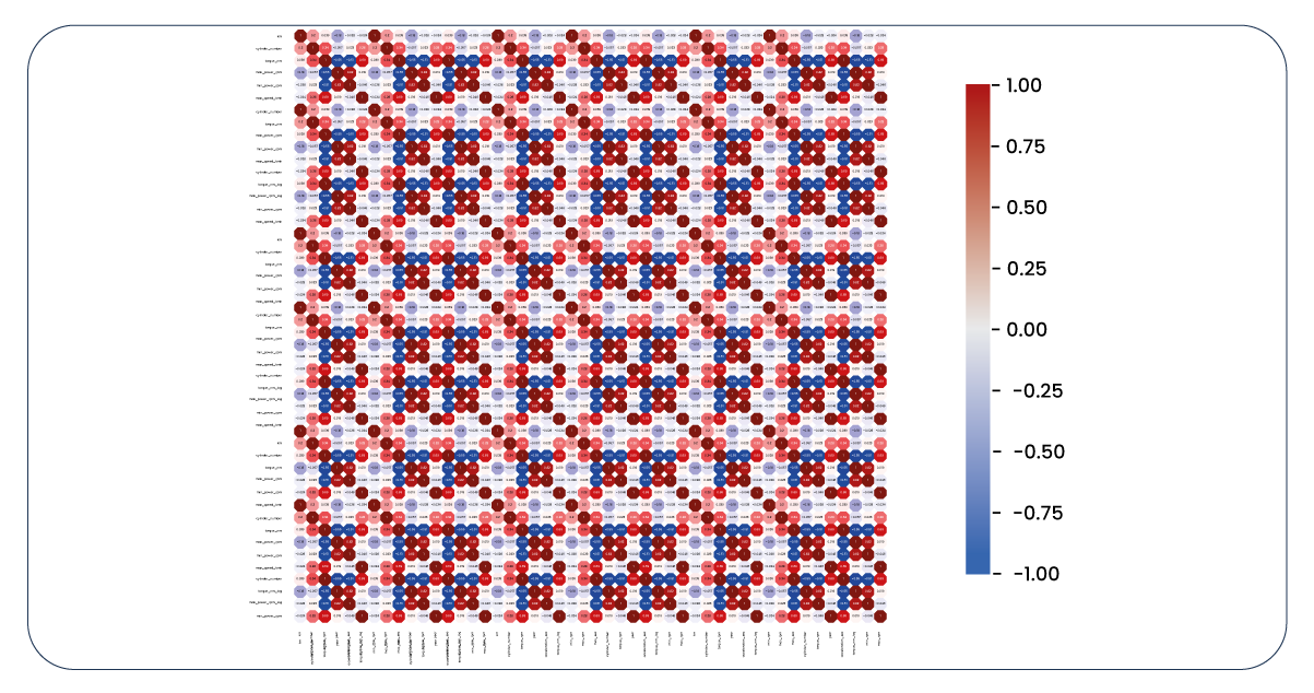
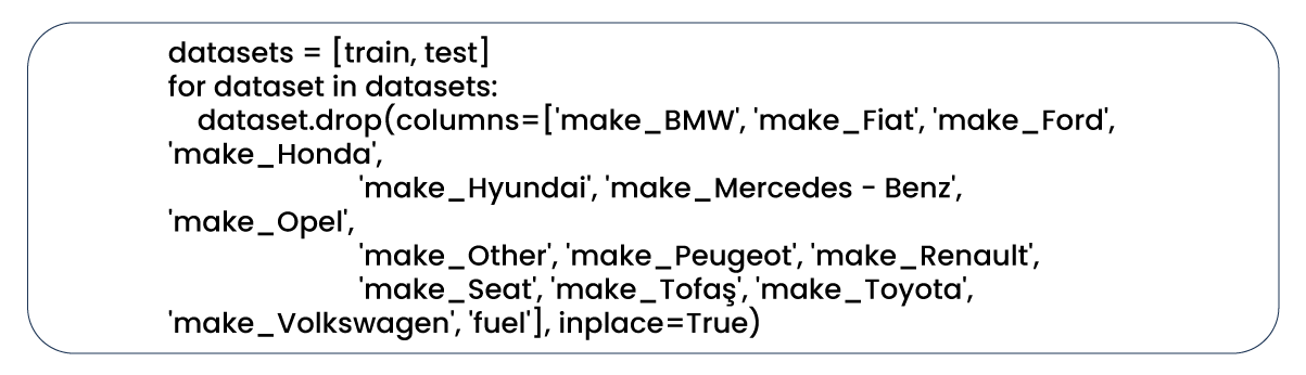
We have extensive features to consider and utilize, which diverges from our initial expectations. After some investigation, it becomes evident that the "make" features are relatively ineffective in predicting the target variable and contribute to multicollinearity issues due to their high correlation with the "series" features. Consequently, it's time to eliminate the "make" column. Additionally, we opt to drop the "fuel" column, as we observe correlations with certain features and a limited impact on the target variable.
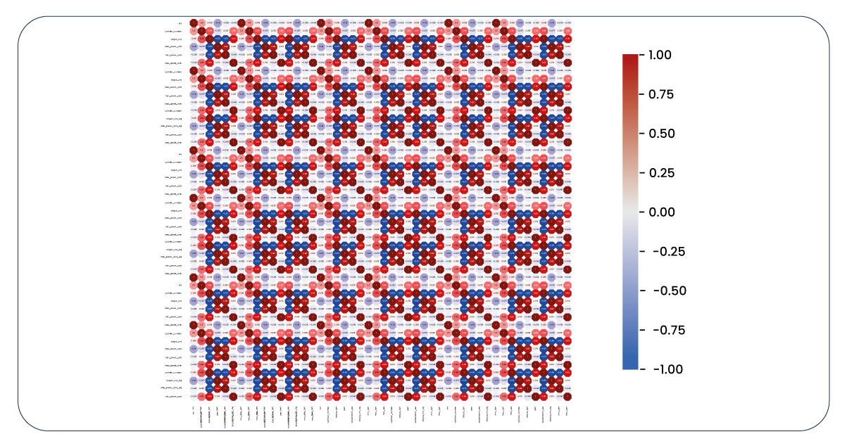
Now, for a final review, let's revisit our correlation heatmap. While it may not be flawless, it now appears more informative and relevant.
Basic Linear Regression and Scaling
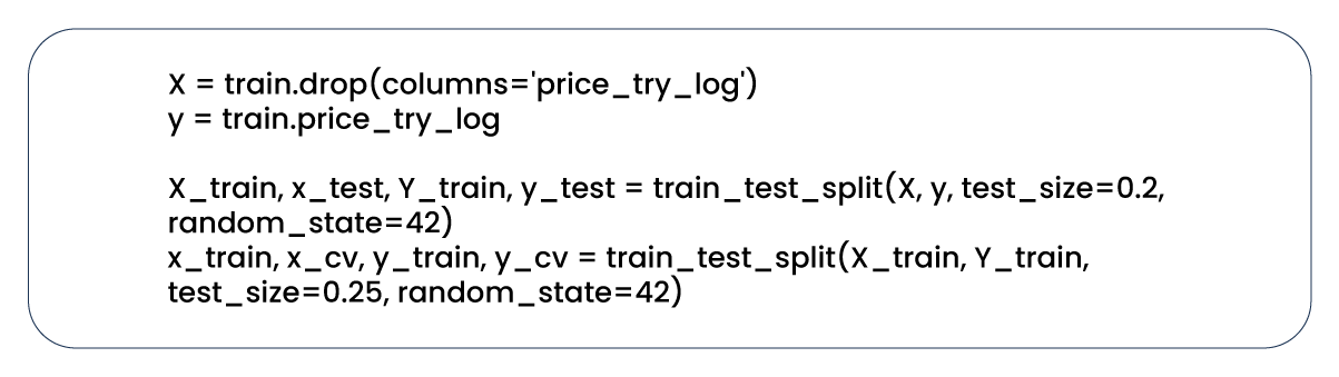
Our initial step involved dividing our data into three sets: 60% for training, 20% for validation, and 20% for testing.
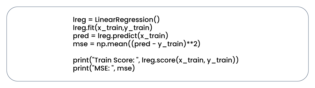
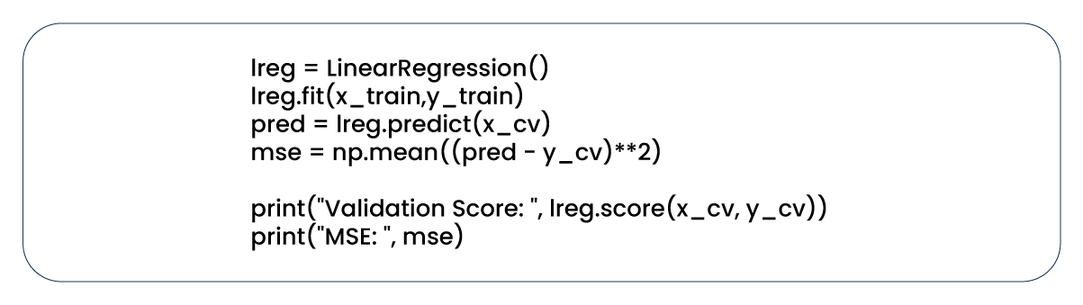
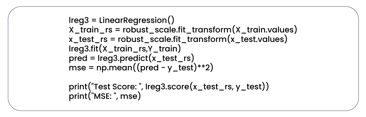
Following the data splitting, we constructed and trained a straightforward linear regression model.
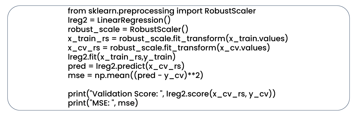
Subsequently, we scaled our data using RobustScaler.
Before and after scaling our data, we achieved an R-squared score of approximately 0.91 with a basic linear regression model, which is reasonably satisfactory. While scaling may have minimal impact initially, its significance will become more apparent during the subsequent regularization and cross-validation stages. Here are the coefficients of our model; while some are relatively high, they are relatively manageable.
Next, we explore the application of Ridge, a commonly employed regularization technique.
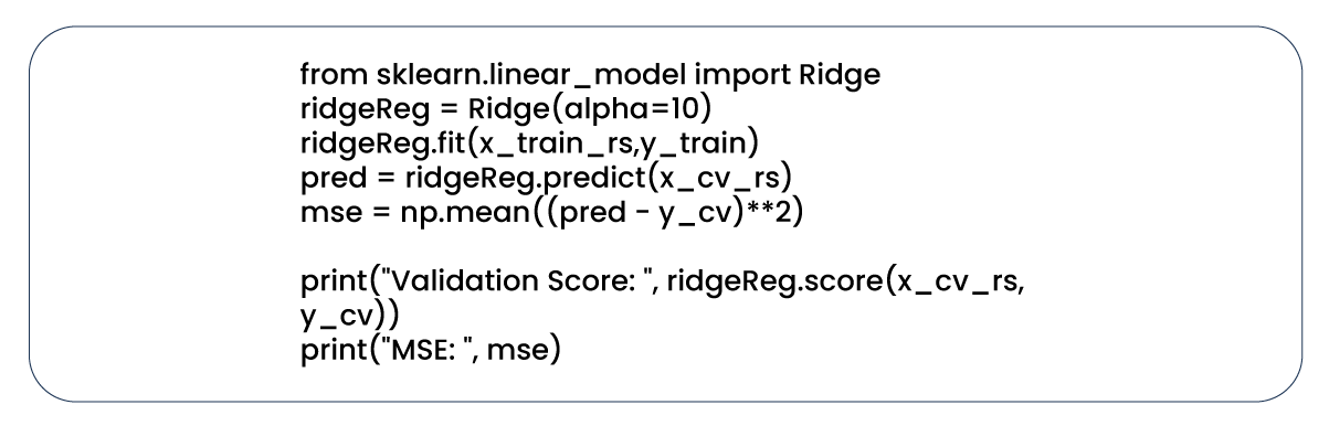
We established a for loop to iterate through various alpha values and identify the one that yields the most favorable results.
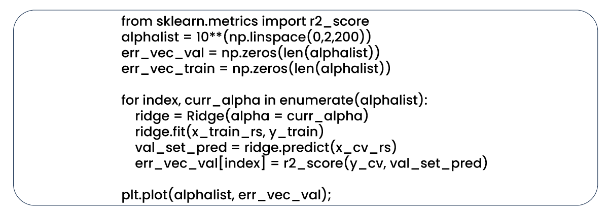
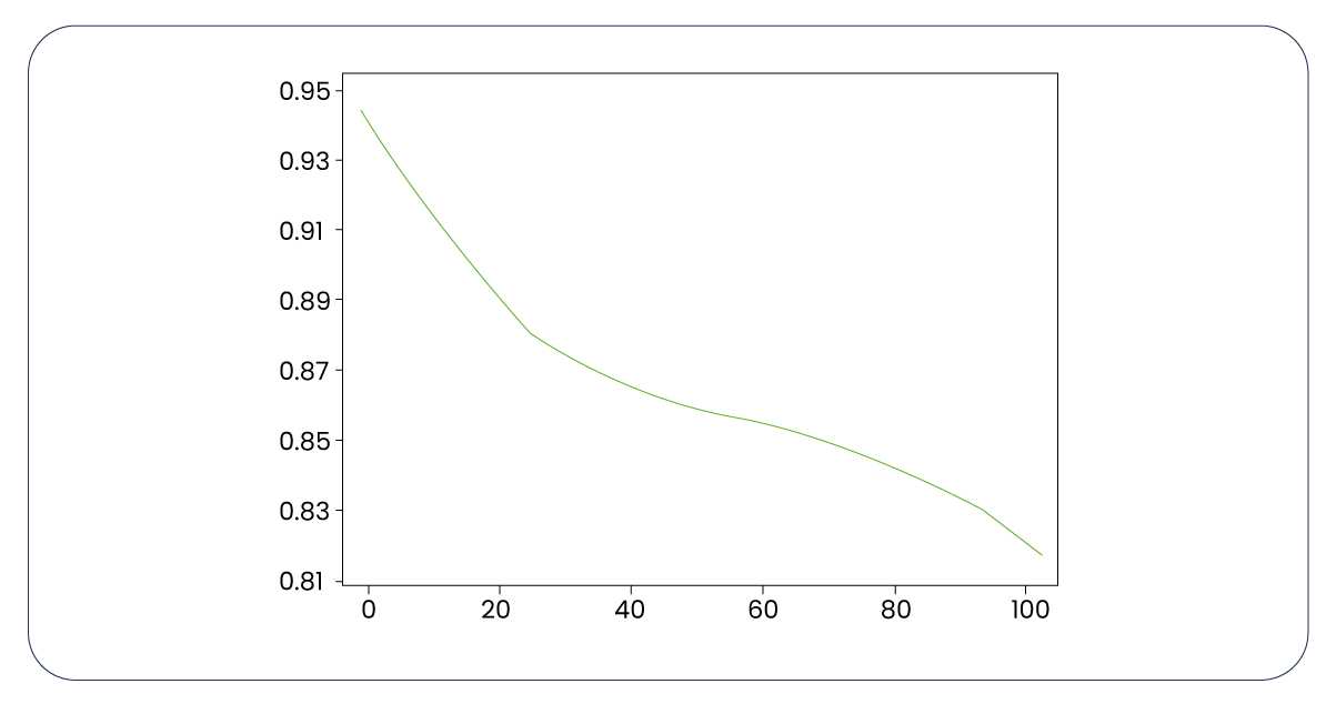
In our model utilizing the Ridge technique, we obtain the highest R-squared score of 0.90 with an alpha value of 1. Additionally, when employing Lasso, another well-known technique, we achieved the highest R-squared score of 0.91.
Cross-Validation
We are embarking on implementing cross-validation, a pivotal stage in the machine learning modeling process. Before our initial data splitting into 60%, 20%, and 20%, we had divided our train dataset into 80% and 20%. We further partition this 80% portion into ten parts for cross-validation purposes. We individually replicate this process for linear regression, Ridge, and Lasso models.
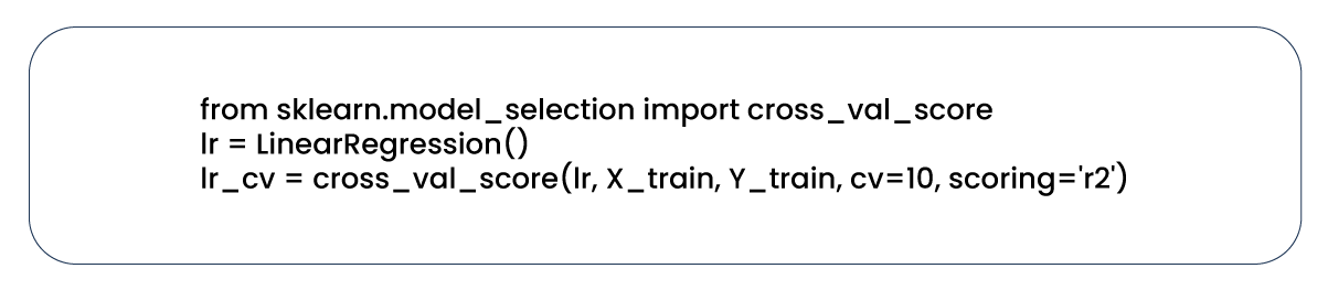
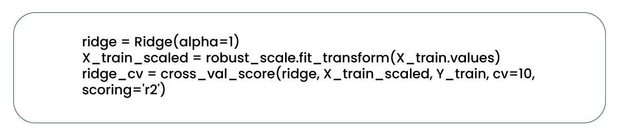
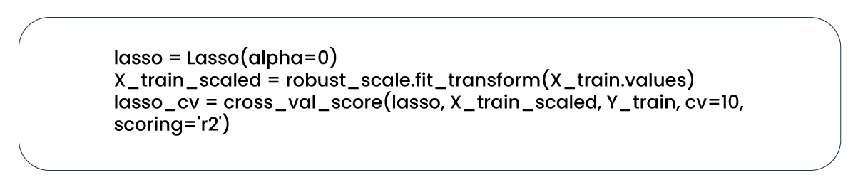
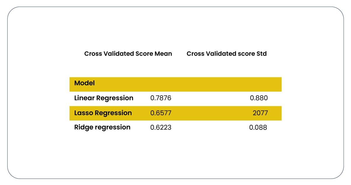
Following cross-validation, we computed the R-squared scores' means and standard deviations.
We've reached the final stage of the modeling process, where we can employ our test dataset for car price predictions. It's worth noting that in the feature engineering phase, we took the logarithms of the values in the "price_try" column, and at this point, we need to reverse that transformation.

Here are a few instances of predictions made by our model.
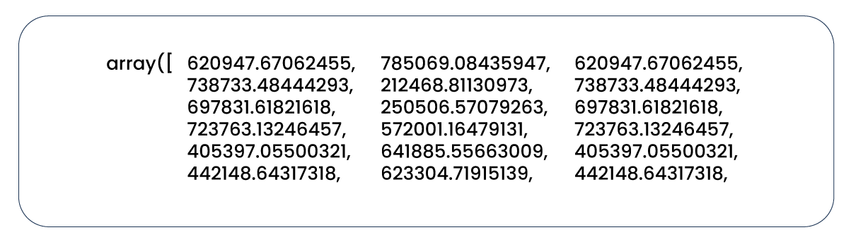
Lastly, we aimed to visualize the predictions generated by our model using a data frame.



 Singapore
 EMAIL
EMAIL
 PHONE
PHONE


.webp)















.webp)